import datetime as dt
from datetime import timedelta
import sys, os
import pandas as pd
import numpy as np
from tqdm import tqdm
from pathlib import Path
import matplotlib.pyplot as plt

from viresclient import set_token
sys.path.append("..")
import utilities
from utilities.MagGeoFunctions import getGPSData
from utilities.MagGeoFunctions import Get_Swarm_residualsMagGeo - Parallel Mode
Authors | Fernando Benitez-Paez, Urška Demšar, Jed Long, Ciaran Beggan
Contact | Fernando.Benitez@st-andrews.ac.uk, ud2@st-andrews.ac.uk, jed.long@uwo.ca, ciar@bgs.ac.uk
Keywords | Bird migration, data fusion, Earth’s magnetic field, Swarm, GPS tracking
Overview
This Jupyter Notebook will guide you through the required steps to annotate your GPS tracking data with the earth’s magnetic field data from Swarm (European Space Agency). This version is called Parallel Mode to take advantage of parallelized computing to process big datasets.
To execute the code, you can go through each cell (pressing Crtl+Enter), you will also find inner comments ## to describe each particular step. If you are not familiar with Jupyter Notebook, you migth want to take some time to learn how to use it first, for example take a look at the notebook-basics.ipynb Notebook inside MagGeo.
For parallel processing, there are some considerations to make:
- Linux and Windows environments have some differences. In windows we need to separate the functions and store them separately, then import them into a
mainfunction. - Defining what part of the process is CPU bound and what part is I/O bound: Identify what parts of the program are I/O bound (writing or reading from the disk or network) and what part par CPU bound ( Processing capacity). To take advantage of our CPU capacity we need to identify the process where the CPU is actually doing the main Tasks.
Data requirements
🔎 Your trajectory must be in a csv format:
There are three columns that must be included in your GPS trajectory. Make sure your GPS trajectory includes Latitude , Longitude and timestamp. We suggest that the Timestamp column follow the day/month/year Hour:Minute (dd/mm/yyyy HH:MM:SS) format, Latitude and Longitude should be in decimal degrees (WGS84). Optionally an altitude column can be used providing altitude (the altitude must be in km). Other Columns will be ignored. Here it is an example of how your GPS track should look:

For this example we are reading the BirdGPSTrajectory.csv file. If you want to run the method using your own csv file, make sure you store your the file in the ./data folder. For more information about the dataset we used in this example go to the Main Notebook.
Import the requeried libraries
Add your VirES web client Token
The VirES client API, requires a token. Before start you need to get your own VirES token. You can visit https://vires.services/ to get yours, and then add it into the next cell.
set_token("https://vires.services/ows", set_default=True)Reading the GPS track
The following steps will load the GPS track from a csv file, and set some requirements before download the data from Swarm. Importing the GPS track. You can note that there is a folder to store the CSV file. Using os.getcwd() you can validate where the file is located.
base_dir=os.path.dirname(os.getcwd())
temp_results_dir = os.path.join(base_dir, "temp_data")
results_dir = os.path.join(base_dir, "results")
data_dir = os.path.join(base_dir, "data")
#Make sure the csv file of your trackectory is stored in the Data folder.
#Enter the name of your GPS track csv file including the extension .csv and press Enter (e.g. BirdGPSTrajectory.csv)
# Make sure you have a columnn that integrates date and time, before include in MagGeo.
#If your csv track file does not have any altitude attribute, MagGeo will use sea level as your altitude (i.e. 0 Km).
# i.e height (Only in KM)
gpsfilename= "BirdGPSTrajectoryTest.csv"
Lat="location-lat"
Long="location-long"
DateTime="timestamp"
altitude = "height"# Here MagGeo is reading your CSV file, taking the Lat, Long, Date&Time and Altitutes attributes and compute, some aditional attrubutes we need to the annotation process.
# Setting the date and time attributes for the required format and computing the epoch column. Values like Maximum and Minimun Date and time are also calculated.
GPSData = getGPSData(data_dir,gpsfilename,Lat,Long,DateTime,altitude)
GPSData| gpsDateTime | gpsLong | gpsLat | gpsAltitude | epoch | dates | times | |
|---|---|---|---|---|---|---|---|
| 0 | 2014-09-08 05:54:00 | 68.307333 | 70.854717 | 0.000 | 1410155640 | 2014-09-08 | 05:54:00 |
| 1 | 2014-09-08 06:10:00 | 67.975050 | 70.830300 | 0.406 | 1410156600 | 2014-09-08 | 06:10:00 |
| 2 | 2014-09-08 06:26:00 | 67.752417 | 70.761717 | 0.498 | 1410157560 | 2014-09-08 | 06:26:00 |
| 3 | 2014-09-08 06:42:00 | 67.561983 | 70.686517 | 0.787 | 1410158520 | 2014-09-08 | 06:42:00 |
| 4 | 2014-09-08 07:14:00 | 67.548317 | 70.685450 | 0.337 | 1410160440 | 2014-09-08 | 07:14:00 |
| ... | ... | ... | ... | ... | ... | ... | ... |
| 194 | 2014-09-27 11:09:00 | 49.503800 | 67.735100 | 0.098 | 1411816140 | 2014-09-27 | 11:09:00 |
| 195 | 2014-09-27 11:25:00 | 49.503767 | 67.735100 | 0.099 | 1411817100 | 2014-09-27 | 11:25:00 |
| 196 | 2014-09-27 11:40:00 | 49.503667 | 67.735100 | 0.100 | 1411818000 | 2014-09-27 | 11:40:00 |
| 197 | 2014-09-27 11:56:00 | 49.503650 | 67.735100 | 0.100 | 1411818960 | 2014-09-27 | 11:56:00 |
| 198 | 2014-09-27 12:11:00 | 49.503617 | 67.735000 | 0.092 | 1411819860 | 2014-09-27 | 12:11:00 |
199 rows × 7 columns
Setting the date and time attributes for the requerided format and computing the epoch column. Values like Maximum and Minimun Date and time are also calculated.
Validate the right amount of Swarm measures
The following loop is identifiying the time and validating if the time is less than 4:00 hours and more than 20:00 hours to bring one extra day of data. The result of this validation is written in a empty python list which will be later validated to get the unique dates avoing to download data for the same day and reducing the the downloand time process.
%%time
datestimeslist = []
for index, row in GPSData.iterrows():
    datetimerow  = row['gpsDateTime']
    daterow = row['dates']
    hourrow = row['times']
    hourrow = hourrow.strftime('%H:%M:%S')
    if hourrow < '04:00:00':
        date_bfr = daterow - (timedelta(days=1))
        datestimeslist.append(daterow)
        datestimeslist.append(date_bfr)
    if hourrow > '20:00:00':
        Date_aft = daterow + (timedelta(days=1))
        datestimeslist.append(daterow)
        datestimeslist.append(Date_aft)
    else:
        datestimeslist.append(daterow)
Getting a list of unique dates, to being used to download the Swarm Data
%%time
def uniquelistdates(list):
    x = np.array(list)
    uniquelist = np.unique(x)
    return uniquelist

uniquelist_dates = uniquelistdates(datestimeslist)
uniquelist_dates
Download Swarm residuals data
Once the date and time columns have been defined, and the unique dates were identified the script can start the download process. Usually the data from Swarm is requested using only one satellite, however MagGeo will use the magnetic measures from the three satellite of the Swarm Mission.
📘 Be aware: Due to the amount of dates the GPS track has (42 days) to request and compute the residuals, the time to process the sample data will take approximately 10 minutes.
Set a connection to the VirES client and using the function Get_Swarm_residuals we will get the swarm residuals for the dates included in the previous list.
%%time

hours_t_day = 24
hours_added = dt.timedelta(hours = hours_t_day)

listdfa = []
listdfb = []
listdfc = []

for d in tqdm(uniquelist_dates, desc="Getting Swarm Data"):
    #print("Getting Swarm data for date:",d )
    startdate = dt.datetime.combine(d, dt.datetime.min.time())
    enddate = startdate + hours_added
    SwarmResidualsA,SwarmResidualsB,SwarmResidualsC = Get_Swarm_residuals(startdate, enddate)
    listdfa.append(SwarmResidualsA)
    listdfb.append(SwarmResidualsB)
    listdfc.append(SwarmResidualsC)
Concat the previous results and temporally save the requested data locally: Integrate the previous list for all dates, into pandas dataframes. We will temporally saved the previous results, in case you need to re-run MagGeo, with the following csv files you will not need to run the download process.
%%time
TotalSwarmRes_A = pd.concat(listdfa, join='outer', axis=0)
TotalSwarmRes_A.to_csv (os.path.join(temp_results_dir,'TotalSwarmRes_A.csv'), header=True)
TotalSwarmRes_B = pd.concat(listdfb, join='outer', axis=0)
TotalSwarmRes_B.to_csv (os.path.join(temp_results_dir,'TotalSwarmRes_B.csv'), header=True)
TotalSwarmRes_C = pd.concat(listdfc, join='outer', axis=0)
TotalSwarmRes_C.to_csv (os.path.join(temp_results_dir,'TotalSwarmRes_C.csv'), header=True)
TotalSwarmRes_A #If you need to take a look of the Swarm Data, you can print TotalSwarmRes_B, or TotalSwarmRes_C
Set the number of processes, and split the dataframe (GPSData) into chunks
We can set the number or processess we need to dedicate for the multiprocessing mode, of course that also depends on the number of cores the machine you are using to run MagGeo. You can use multiprocessing.cpu_count() to set the number of processes as the the number of cores your machine has. Beside that we will also to split the GPS track into chucks to dedicate each core for each chuck. For more information take a look at the Home Notebook.
import multiprocessing
import sklearn
from multiprocessing import Pool

NumCores = multiprocessing.cpu_count()
df_chunks = np.array_split(GPSData,NumCores)
df_chunks
[ gpsDateTime gpsLong gpsLat gpsAltitude epoch \
0 2014-09-08 05:54:00 68.307333 70.854717 0.000 1410155640
1 2014-09-08 06:10:00 67.975050 70.830300 0.406 1410156600
2 2014-09-08 06:26:00 67.752417 70.761717 0.498 1410157560
3 2014-09-08 06:42:00 67.561983 70.686517 0.787 1410158520
4 2014-09-08 07:14:00 67.548317 70.685450 0.337 1410160440
5 2014-09-08 07:30:00 67.549433 70.685750 0.026 1410161400
6 2014-09-08 07:46:00 67.530983 70.690333 0.026 1410162360
7 2014-09-08 08:03:00 67.506233 70.692683 0.023 1410163380
8 2014-09-08 08:34:00 67.506167 70.692533 0.022 1410165240
9 2014-09-08 08:50:00 67.506383 70.692583 0.023 1410166200
10 2014-09-08 09:37:00 67.501633 70.695017 0.026 1410169020
11 2014-09-08 09:54:00 67.498917 70.693850 0.026 1410170040
12 2014-09-08 13:53:00 67.505800 70.692667 0.000 1410184380
dates times
0 2014-09-08 05:54:00
1 2014-09-08 06:10:00
2 2014-09-08 06:26:00
3 2014-09-08 06:42:00
4 2014-09-08 07:14:00
5 2014-09-08 07:30:00
6 2014-09-08 07:46:00
7 2014-09-08 08:03:00
8 2014-09-08 08:34:00
9 2014-09-08 08:50:00
10 2014-09-08 09:37:00
11 2014-09-08 09:54:00
12 2014-09-08 13:53:00 ,
gpsDateTime gpsLong gpsLat gpsAltitude epoch \
13 2014-09-08 14:09:00 67.505883 70.692667 0.034 1410185340
14 2014-09-08 14:25:00 67.506000 70.692617 0.034 1410186300
15 2014-09-08 14:41:00 67.505883 70.692750 0.033 1410187260
16 2014-09-08 15:13:00 67.511617 70.694350 0.036 1410189180
17 2014-09-08 15:29:00 67.509050 70.693650 0.034 1410190140
18 2014-09-08 15:45:00 67.511250 70.693467 0.032 1410191100
19 2014-09-08 16:01:00 67.510000 70.693450 0.033 1410192060
20 2014-09-08 16:33:00 67.510767 70.693633 0.034 1410193980
21 2014-09-08 16:49:00 67.509500 70.693583 0.033 1410194940
22 2014-09-08 17:05:00 67.509750 70.693600 0.033 1410195900
23 2014-09-08 17:38:00 67.509700 70.693633 0.035 1410197880
24 2014-09-08 17:53:00 67.509650 70.693650 0.017 1410198780
25 2014-09-21 12:23:00 49.996717 66.897217 0.019 1411302180
dates times
13 2014-09-08 14:09:00
14 2014-09-08 14:25:00
15 2014-09-08 14:41:00
16 2014-09-08 15:13:00
17 2014-09-08 15:29:00
18 2014-09-08 15:45:00
19 2014-09-08 16:01:00
20 2014-09-08 16:33:00
21 2014-09-08 16:49:00
22 2014-09-08 17:05:00
23 2014-09-08 17:38:00
24 2014-09-08 17:53:00
25 2014-09-21 12:23:00 ,
gpsDateTime gpsLong gpsLat gpsAltitude epoch \
26 2014-09-21 12:55:00 49.997550 66.897567 0.030 1411304100
27 2014-09-21 13:11:00 49.998683 66.898600 0.000 1411305060
28 2014-09-21 13:43:00 49.997133 66.898300 0.000 1411306980
29 2014-09-21 14:00:00 49.997383 66.897600 0.000 1411308000
30 2014-09-21 14:17:00 49.997467 66.897517 0.000 1411309020
31 2014-09-21 14:31:00 50.005250 66.895483 0.044 1411309860
32 2014-09-21 15:03:00 50.040800 66.890583 0.000 1411311780
33 2014-09-21 15:19:00 50.047867 66.890167 0.000 1411312740
34 2014-09-21 15:35:00 50.047600 66.890150 0.000 1411313700
35 2014-09-21 16:07:00 50.047800 66.890183 0.000 1411315620
36 2014-09-21 16:23:00 49.961467 66.980783 0.000 1411316580
37 2014-09-22 05:52:00 49.847017 66.960383 0.000 1411365120
38 2014-09-22 06:08:00 49.846967 66.960450 0.000 1411366080
dates times
26 2014-09-21 12:55:00
27 2014-09-21 13:11:00
28 2014-09-21 13:43:00
29 2014-09-21 14:00:00
30 2014-09-21 14:17:00
31 2014-09-21 14:31:00
32 2014-09-21 15:03:00
33 2014-09-21 15:19:00
34 2014-09-21 15:35:00
35 2014-09-21 16:07:00
36 2014-09-21 16:23:00
37 2014-09-22 05:52:00
38 2014-09-22 06:08:00 ,
gpsDateTime gpsLong gpsLat gpsAltitude epoch \
39 2014-09-22 06:24:00 49.846950 66.960367 0.000 1411367040
40 2014-09-22 06:40:00 49.847350 66.960383 0.000 1411368000
41 2014-09-22 07:13:00 49.846850 66.960400 0.000 1411369980
42 2014-09-22 08:02:00 49.712750 67.096717 0.000 1411372920
43 2014-09-30 06:35:00 47.120217 66.684717 0.006 1412058900
44 2014-09-30 06:51:00 46.696433 66.529533 0.000 1412059860
45 2014-09-30 07:07:00 46.267167 66.378733 0.000 1412060820
46 2014-09-30 07:23:00 45.813017 66.230733 0.000 1412061780
47 2014-09-30 08:04:00 44.659750 65.770600 0.000 1412064240
48 2014-09-30 08:46:00 43.495867 65.287350 0.000 1412066760
49 2014-09-30 10:10:00 41.314500 64.129950 0.000 1412071800
50 2014-09-30 10:26:00 40.957017 63.896433 0.000 1412072760
51 2014-09-30 11:04:00 40.313267 63.317133 0.000 1412075040
dates times
39 2014-09-22 06:24:00
40 2014-09-22 06:40:00
41 2014-09-22 07:13:00
42 2014-09-22 08:02:00
43 2014-09-30 06:35:00
44 2014-09-30 06:51:00
45 2014-09-30 07:07:00
46 2014-09-30 07:23:00
47 2014-09-30 08:04:00
48 2014-09-30 08:46:00
49 2014-09-30 10:10:00
50 2014-09-30 10:26:00
51 2014-09-30 11:04:00 ,
gpsDateTime gpsLong gpsLat gpsAltitude epoch \
52 2014-09-30 11:21:00 40.012267 63.049433 0.0 1412076060
53 2014-09-30 11:53:00 39.520267 62.547750 0.0 1412077980
54 2014-09-30 12:09:00 39.286400 62.327483 0.0 1412078940
55 2014-09-30 16:27:00 35.165983 59.422467 0.0 1412094420
56 2014-09-30 16:59:00 34.759200 58.980250 0.0 1412096340
57 2014-09-30 17:15:00 34.471817 58.817917 0.0 1412097300
58 2014-09-30 17:47:00 34.448300 58.827933 0.0 1412099220
59 2014-09-30 18:04:00 34.448467 58.826017 0.0 1412100240
60 2014-09-30 18:20:00 34.435233 58.819850 0.0 1412101200
61 2014-09-30 18:35:00 34.201167 58.727250 0.0 1412102100
62 2014-09-30 19:08:00 33.569233 58.405500 0.0 1412104080
63 2014-09-30 19:24:00 33.236700 58.241183 0.0 1412105040
64 2014-09-30 19:40:00 33.014350 58.041567 0.0 1412106000
dates times
52 2014-09-30 11:21:00
53 2014-09-30 11:53:00
54 2014-09-30 12:09:00
55 2014-09-30 16:27:00
56 2014-09-30 16:59:00
57 2014-09-30 17:15:00
58 2014-09-30 17:47:00
59 2014-09-30 18:04:00
60 2014-09-30 18:20:00
61 2014-09-30 18:35:00
62 2014-09-30 19:08:00
63 2014-09-30 19:24:00
64 2014-09-30 19:40:00 ,
gpsDateTime gpsLong gpsLat gpsAltitude epoch \
65 2014-09-30 19:56:00 32.698767 57.913150 0.000 1412106960
66 2014-09-30 20:12:00 32.470350 57.709567 0.003 1412107920
67 2014-09-30 20:28:00 32.223617 57.567683 0.002 1412108880
68 2014-10-01 00:29:00 31.970950 57.454033 0.000 1412123340
69 2014-10-01 00:44:00 31.971250 57.453767 0.000 1412124240
70 2014-10-01 01:00:00 31.971667 57.453667 0.037 1412125200
71 2014-10-01 02:42:00 31.894067 57.427383 0.038 1412131320
72 2014-10-01 02:59:00 31.669200 57.321483 0.128 1412132340
73 2014-10-01 03:14:00 31.446667 57.195767 0.135 1412133240
74 2014-10-01 05:05:00 29.696600 56.703217 0.131 1412139900
75 2014-10-01 06:19:00 28.411983 56.252417 0.127 1412144340
76 2014-10-01 06:35:00 28.150767 56.085417 0.132 1412145300
77 2014-10-01 07:23:00 27.264867 55.628233 0.132 1412148180
dates times
65 2014-09-30 19:56:00
66 2014-09-30 20:12:00
67 2014-09-30 20:28:00
68 2014-10-01 00:29:00
69 2014-10-01 00:44:00
70 2014-10-01 01:00:00
71 2014-10-01 02:42:00
72 2014-10-01 02:59:00
73 2014-10-01 03:14:00
74 2014-10-01 05:05:00
75 2014-10-01 06:19:00
76 2014-10-01 06:35:00
77 2014-10-01 07:23:00 ,
gpsDateTime gpsLong gpsLat gpsAltitude epoch \
78 2014-10-01 07:40:00 26.967033 55.513917 0.132 1412149200
79 2014-10-01 07:56:00 26.703400 55.396383 0.131 1412150160
80 2014-10-01 11:42:00 22.913617 53.929300 0.129 1412163720
81 2014-10-01 12:13:00 22.347700 53.795100 0.131 1412165580
82 2014-10-01 12:29:00 22.068817 53.726433 0.129 1412166540
83 2014-10-01 13:02:00 21.519500 53.613633 0.000 1412168520
84 2014-10-01 13:18:00 21.238517 53.580000 0.142 1412169480
85 2014-10-01 13:34:00 20.974200 53.522383 0.137 1412170440
86 2014-10-01 13:50:00 20.682200 53.486600 0.136 1412171400
87 2014-10-01 14:22:00 20.148067 53.381400 0.000 1412173320
88 2014-10-01 14:38:00 19.858717 53.353933 0.134 1412174280
89 2014-10-01 14:54:00 19.568867 53.324533 0.149 1412175240
90 2014-10-01 15:26:00 18.964567 53.259633 0.145 1412177160
dates times
78 2014-10-01 07:40:00
79 2014-10-01 07:56:00
80 2014-10-01 11:42:00
81 2014-10-01 12:13:00
82 2014-10-01 12:29:00
83 2014-10-01 13:02:00
84 2014-10-01 13:18:00
85 2014-10-01 13:34:00
86 2014-10-01 13:50:00
87 2014-10-01 14:22:00
88 2014-10-01 14:38:00
89 2014-10-01 14:54:00
90 2014-10-01 15:26:00 ,
gpsDateTime gpsLong gpsLat gpsAltitude epoch \
91 2014-10-01 15:42:00 18.664850 53.268217 0.145 1412178120
92 2014-10-01 19:42:00 16.177583 53.797867 0.143 1412192520
93 2014-10-01 19:57:00 16.178717 53.798633 0.136 1412193420
94 2014-10-01 20:13:00 16.179067 53.798667 0.135 1412194380
95 2014-10-01 20:30:00 16.179150 53.798850 0.133 1412195400
96 2014-10-01 21:02:00 16.178950 53.798350 0.134 1412197320
97 2014-10-01 21:18:00 16.178817 53.798350 0.146 1412198280
98 2014-10-01 21:34:00 16.179200 53.798467 0.124 1412199240
99 2014-10-01 21:50:00 16.178483 53.798617 0.117 1412200200
100 2014-10-01 22:22:00 16.179033 53.798367 0.118 1412202120
101 2014-10-01 22:38:00 16.178983 53.797933 0.119 1412203080
102 2014-10-01 23:10:00 16.178733 53.798333 0.118 1412205000
dates times
91 2014-10-01 15:42:00
92 2014-10-01 19:42:00
93 2014-10-01 19:57:00
94 2014-10-01 20:13:00
95 2014-10-01 20:30:00
96 2014-10-01 21:02:00
97 2014-10-01 21:18:00
98 2014-10-01 21:34:00
99 2014-10-01 21:50:00
100 2014-10-01 22:22:00
101 2014-10-01 22:38:00
102 2014-10-01 23:10:00 ,
gpsDateTime gpsLong gpsLat gpsAltitude epoch \
103 2014-10-01 23:26:00 16.178650 53.798483 0.126 1412205960
104 2014-10-01 23:42:00 16.179417 53.798400 0.129 1412206920
105 2014-10-01 23:58:00 16.179233 53.798633 0.107 1412207880
106 2014-10-02 03:42:00 16.179567 53.795533 0.108 1412221320
107 2014-10-02 04:14:00 16.161283 53.889767 0.109 1412223240
108 2014-10-02 05:02:00 15.977883 54.208517 0.913 1412226120
109 2014-10-02 05:18:00 15.791683 54.210117 0.823 1412227080
110 2014-10-02 05:35:00 15.640317 54.180867 0.010 1412228100
111 2014-10-02 05:51:00 15.502350 54.150750 0.005 1412229060
112 2014-10-02 06:22:00 15.502000 54.150600 0.009 1412230920
113 2014-10-02 06:38:00 15.500733 54.145917 0.000 1412231880
114 2014-10-02 07:26:00 15.500717 54.146000 0.000 1412234760
dates times
103 2014-10-01 23:26:00
104 2014-10-01 23:42:00
105 2014-10-01 23:58:00
106 2014-10-02 03:42:00
107 2014-10-02 04:14:00
108 2014-10-02 05:02:00
109 2014-10-02 05:18:00
110 2014-10-02 05:35:00
111 2014-10-02 05:51:00
112 2014-10-02 06:22:00
113 2014-10-02 06:38:00
114 2014-10-02 07:26:00 ,
gpsDateTime gpsLong gpsLat gpsAltitude epoch \
115 2014-10-02 07:43:00 15.499767 54.145750 0.000 1412235780
116 2014-10-02 11:43:00 15.236950 54.089233 0.000 1412250180
117 2014-10-02 11:59:00 15.236767 54.089383 0.003 1412251140
118 2014-10-02 12:15:00 15.236850 54.089300 0.005 1412252100
119 2014-10-02 12:31:00 15.236900 54.089283 0.381 1412253060
120 2014-10-02 13:04:00 15.236850 54.089267 0.928 1412255040
121 2014-10-02 13:20:00 15.236750 54.089433 0.337 1412256000
122 2014-10-02 13:36:00 15.236067 54.090017 0.267 1412256960
123 2014-10-02 13:52:00 15.236983 54.089300 0.357 1412257920
124 2014-10-02 14:24:00 15.237417 54.089350 0.140 1412259840
125 2014-10-02 14:41:00 15.236900 54.089200 0.315 1412260860
126 2014-10-02 14:57:00 15.237067 54.089250 0.132 1412261820
dates times
115 2014-10-02 07:43:00
116 2014-10-02 11:43:00
117 2014-10-02 11:59:00
118 2014-10-02 12:15:00
119 2014-10-02 12:31:00
120 2014-10-02 13:04:00
121 2014-10-02 13:20:00
122 2014-10-02 13:36:00
123 2014-10-02 13:52:00
124 2014-10-02 14:24:00
125 2014-10-02 14:41:00
126 2014-10-02 14:57:00 ,
gpsDateTime gpsLong gpsLat gpsAltitude epoch \
127 2014-10-02 15:29:00 15.236800 54.088833 0.136 1412263740
128 2014-10-02 15:45:00 15.237250 54.090200 0.133 1412264700
129 2014-10-02 19:45:00 15.111483 54.130650 0.133 1412279100
130 2014-10-02 20:01:00 15.111733 54.131350 0.130 1412280060
131 2014-10-02 20:17:00 15.111050 54.132650 0.133 1412281020
132 2014-10-02 20:34:00 15.109267 54.131633 0.133 1412282040
133 2014-10-02 21:06:00 15.107017 54.133217 0.132 1412283960
134 2014-10-02 21:22:00 15.106033 54.133567 0.128 1412284920
135 2014-10-02 21:38:00 15.103083 54.134050 0.124 1412285880
136 2014-10-02 21:54:00 15.101467 54.133400 0.129 1412286840
137 2014-10-02 22:26:00 15.096867 54.132917 0.132 1412288760
138 2014-10-02 22:42:00 15.093067 54.133083 0.130 1412289720
dates times
127 2014-10-02 15:29:00
128 2014-10-02 15:45:00
129 2014-10-02 19:45:00
130 2014-10-02 20:01:00
131 2014-10-02 20:17:00
132 2014-10-02 20:34:00
133 2014-10-02 21:06:00
134 2014-10-02 21:22:00
135 2014-10-02 21:38:00
136 2014-10-02 21:54:00
137 2014-10-02 22:26:00
138 2014-10-02 22:42:00 ,
gpsDateTime gpsLong gpsLat gpsAltitude epoch \
139 2014-10-02 23:30:00 15.093517 54.138450 0.130 1412292600
140 2014-10-02 23:46:00 15.094350 54.139350 0.133 1412293560
141 2014-10-03 03:47:00 15.093983 54.146717 0.128 1412308020
142 2014-10-03 04:03:00 15.095067 54.147683 0.134 1412308980
143 2014-10-03 04:19:00 15.098000 54.149517 0.128 1412309940
144 2014-10-03 04:35:00 15.104433 54.147617 0.119 1412310900
145 2014-10-03 05:23:00 15.152317 54.096800 0.121 1412313780
146 2014-10-03 05:39:00 15.190917 54.093067 0.132 1412314740
147 2014-10-03 05:55:00 15.197550 54.096967 0.133 1412315700
148 2014-10-03 06:27:00 15.243367 54.089450 0.135 1412317620
149 2014-10-03 06:43:00 15.243600 54.089300 0.135 1412318580
150 2014-10-03 06:59:00 15.244167 54.089067 0.133 1412319540
dates times
139 2014-10-02 23:30:00
140 2014-10-02 23:46:00
141 2014-10-03 03:47:00
142 2014-10-03 04:03:00
143 2014-10-03 04:19:00
144 2014-10-03 04:35:00
145 2014-10-03 05:23:00
146 2014-10-03 05:39:00
147 2014-10-03 05:55:00
148 2014-10-03 06:27:00
149 2014-10-03 06:43:00
150 2014-10-03 06:59:00 ,
gpsDateTime gpsLong gpsLat gpsAltitude epoch \
151 2014-10-03 07:15:00 15.244133 54.089417 0.133 1412320500
152 2014-10-03 07:33:00 15.244200 54.089733 0.133 1412321580
153 2014-10-03 07:47:00 15.243783 54.089867 0.130 1412322420
154 2014-10-03 11:49:00 15.238017 54.089583 0.136 1412336940
155 2014-10-03 12:05:00 15.238167 54.089050 0.158 1412337900
156 2014-10-03 12:22:00 15.238100 54.088700 0.158 1412338920
157 2014-10-03 12:37:00 15.236933 54.088900 0.160 1412339820
158 2014-10-03 13:10:00 15.237350 54.089000 0.162 1412341800
159 2014-10-03 13:26:00 15.237433 54.089017 0.109 1412342760
160 2014-10-03 13:42:00 15.237433 54.088983 0.099 1412343720
161 2014-10-03 13:58:00 15.237433 54.088983 0.106 1412344680
162 2014-10-03 14:30:00 15.236800 54.088517 0.101 1412346600
dates times
151 2014-10-03 07:15:00
152 2014-10-03 07:33:00
153 2014-10-03 07:47:00
154 2014-10-03 11:49:00
155 2014-10-03 12:05:00
156 2014-10-03 12:22:00
157 2014-10-03 12:37:00
158 2014-10-03 13:10:00
159 2014-10-03 13:26:00
160 2014-10-03 13:42:00
161 2014-10-03 13:58:00
162 2014-10-03 14:30:00 ,
gpsDateTime gpsLong gpsLat gpsAltitude epoch \
163 2014-10-03 14:47:00 15.236733 54.088233 0.105 1412347620
164 2014-10-03 15:35:00 15.237633 54.088950 0.101 1412350500
165 2014-10-03 15:51:00 15.243483 54.091083 0.108 1412351460
166 2014-10-03 19:52:00 14.787900 54.018417 0.103 1412365920
167 2014-10-03 20:08:00 14.787250 54.018517 0.104 1412366880
168 2014-10-03 20:24:00 14.786450 54.018783 0.101 1412367840
169 2014-10-03 20:40:00 14.785433 54.019250 0.113 1412368800
170 2014-10-03 21:28:00 14.784967 54.019617 0.127 1412371680
171 2014-10-03 21:44:00 14.786017 54.018650 0.123 1412372640
172 2014-10-03 22:00:00 14.785600 54.018983 0.123 1412373600
173 2014-10-03 22:32:00 14.784983 54.020017 0.104 1412375520
174 2014-10-03 22:48:00 14.785433 54.020367 0.099 1412376480
dates times
163 2014-10-03 14:47:00
164 2014-10-03 15:35:00
165 2014-10-03 15:51:00
166 2014-10-03 19:52:00
167 2014-10-03 20:08:00
168 2014-10-03 20:24:00
169 2014-10-03 20:40:00
170 2014-10-03 21:28:00
171 2014-10-03 21:44:00
172 2014-10-03 22:00:00
173 2014-10-03 22:32:00
174 2014-10-03 22:48:00 ,
gpsDateTime gpsLong gpsLat gpsAltitude epoch \
175 2014-10-03 23:04:00 14.785533 54.020600 0.099 1412377440
176 2014-10-03 23:20:00 14.785650 54.021083 0.098 1412378400
177 2014-10-03 23:36:00 14.785433 54.021517 0.098 1412379360
178 2014-10-03 23:52:00 14.785767 54.021817 0.103 1412380320
179 2014-10-04 03:53:00 14.778733 54.025167 0.103 1412394780
180 2014-10-04 04:09:00 14.778000 54.025550 0.104 1412395740
181 2014-10-04 04:25:00 14.777683 54.025383 0.096 1412396700
182 2014-10-04 04:41:00 14.778167 54.025033 0.104 1412397660
183 2014-10-04 05:29:00 14.780733 53.994583 0.099 1412400540
184 2014-10-04 05:45:00 14.780900 53.994617 0.098 1412401500
185 2014-10-04 06:01:00 14.780883 53.994533 0.099 1412402460
186 2014-10-04 06:33:00 14.780950 53.994300 0.098 1412404380
dates times
175 2014-10-03 23:04:00
176 2014-10-03 23:20:00
177 2014-10-03 23:36:00
178 2014-10-03 23:52:00
179 2014-10-04 03:53:00
180 2014-10-04 04:09:00
181 2014-10-04 04:25:00
182 2014-10-04 04:41:00
183 2014-10-04 05:29:00
184 2014-10-04 05:45:00
185 2014-10-04 06:01:00
186 2014-10-04 06:33:00 ,
gpsDateTime gpsLong gpsLat gpsAltitude epoch \
187 2014-10-04 06:49:00 14.780833 53.994033 0.103 1412405340
188 2014-10-04 07:38:00 14.778800 53.993117 0.103 1412408280
189 2014-10-04 07:53:00 14.718333 53.959217 0.103 1412409180
190 2014-08-30 12:39:00 75.312300 71.454100 0.101 1409402340
191 2014-08-30 14:42:00 75.347050 71.463450 0.102 1409409720
192 2014-08-30 18:49:00 75.379600 71.457583 0.103 1409424540
193 2014-09-27 10:54:00 49.504100 67.734967 0.100 1411815240
194 2014-09-27 11:09:00 49.503800 67.735100 0.098 1411816140
195 2014-09-27 11:25:00 49.503767 67.735100 0.099 1411817100
196 2014-09-27 11:40:00 49.503667 67.735100 0.100 1411818000
197 2014-09-27 11:56:00 49.503650 67.735100 0.100 1411818960
198 2014-09-27 12:11:00 49.503617 67.735000 0.092 1411819860
dates times
187 2014-10-04 06:49:00
188 2014-10-04 07:38:00
189 2014-10-04 07:53:00
190 2014-08-30 12:39:00
191 2014-08-30 14:42:00
192 2014-08-30 18:49:00
193 2014-09-27 10:54:00
194 2014-09-27 11:09:00
195 2014-09-27 11:25:00
196 2014-09-27 11:40:00
197 2014-09-27 11:56:00
198 2014-09-27 12:11:00 ]Spatio-Temporal filter and Interpolation process (ST-IDW)
Once we have requested the swarm data, now we need to filter in space and time the available points to compute the magnetic values (NEC frame) for each GPS point based on its particular date and time. The function ST_IDW_Process imported in the row_handler, takes the GPS track and the downloaded data from swarm to filter in space and time based on the criteria defined in our method. With the swarm data filtered we interpolated (IDW) the NEC components for each GPS data point, based on the latitude, date, time and number of Swarm points filtered.
The function CHAOS_ground_values, inside the MagGeoFunctions file, is used to run the Calculation of magnetic components. This calculation requeries the magnetic components at the trajectory altitude (or at the ground level) using CHAOS (theta, phi, radial). This process include a rotation and transformation between a geocentric frame (CHAOS) and geodetic frame (GPS track). Once the corrected values are calculated, are included in the GPS track, and the non-necesary columns are removed. For more information about this process go to the Main Notebook.
Run the (ST-IDW) process in parallel mode
Although the next cell seems to run a small main function. What is happening is a call for several functions running at same time for several cores. Initially we set a pool of processes. Using the pool class we will distribute the assigned function among the data chucks we created. Every data chunk will be like a subset of the entire GPS track. So we need to iterate among data chunk. And inside every data chunk we need to identify the datetime, epoch, altitude, latitude and longitude of each row to run the interpolation & annotation process using the Swarm data we have filtered and stored in the previous steps.
The function in charge to distribute the required function (row_handler) among the data chunks is the map function from the pool class.
row_handler.py is an interows iteration to get the required parameter for the ST_IDW_Process function.
📘 Auxiliary Functions:
-
ST_IDW_Process function: This is the main function in charge to read the Swarm Data already filtered, and then import
DfTime_func,distance_to_GPS,Kradius,DistJfunctions to compute the spatial-time cylinder and the annotation process. The return of this function is a row (dictionary) that will be appended into a python list where all the results from the different cores. The python list from every process is concatenated into a pandas dataframe in themainfunction having there the whole chain of the parallel process. - distance_to_GPS function: Is the function in charge to calculate the distance between each GPS Point and the Swarm Point.
- Kradius function: Is the function in charge to compute the R (radius) value in the cylinder. The R value will be considered based on the latitude of each GPS Point.
-
DistJ function: This function will calculate the
dvalue as the hypotenuse created in the triangle created amount the locations of the GPS point, the location of the Swarm points and the radius value. -
DfTime_func function: This is a time function to selected the points in the range of a the DeltaTime -
DTwindow. The Delta time window has been set as 4 hours for each satellite trajectory. - CHAOS_ground_values function: This is the calculation of geomagnetic components function to get the CHAOS magnetic values and process the Nres,Eres,Cres values and transform them into the N,E,C values at the GPS altitude.
%%time
from functools import partial
from utilities.row_handler import row_handler

if __name__ == '__main__':
    with multiprocessing.Pool(NumCores) as pool:
        GeoMagParallelResult = pd.concat(pool.map(partial(row_handler),df_chunks), ignore_index=True)
Annotating the GPS Trayectory: 100%|██████████| 12/12 [00:00<00:00, 18.64it/s]
CPU times: user 245 ms, sys: 265 ms, total: 510 ms
Wall time: 17.5 s
With the Parallel mode the Annotation process takes about 12 seconds to complete ( We had tested the parallel process in a windows server machine with 12 cores, see the image bellow). With the same GPS track in the sequetial mode the process is complete in about 2 minutes. In the image bellow you can see how the machine create several python processes and all cores (full CPU capacity) is taken.
🔈 Multiprocessing:
is even more powerfull when you have to process a big amount of data (e.g. 2 millons of points). Although here is making a notable improvement if you have to process a big dataset the parallelization makes even more sense.
Be aware that there is no output cell in here, you can follow the parallelization progress in the Anaconda Prompt.

The final result
With the NEC components for each GPS Track point, it is possible to compute the aditional magnetic components. For more information about the magnetic components and their relevance go to the main paper or notebook.
<strong>📘 The annotated dataframe will include the following attributes:</strong> If you need more information about how the geomagnetic component are described go to the main MagGeo Notebook (Add Link).
<ul>
  <li><strong>Latitude</strong> from the GPS Track.</li>
  <li><strong>Longitude</strong> from the GPS Track.</li>
  <li><strong>Timestamp</strong> from the GPS Track.</li>
  <li><strong>Magnetic Field Intensity</strong>  mapped as Fgps in nanoTeslas (nT).</li>
  <li><strong>N (Northwards) component</strong> mapped as N in nanoTeslas (nT).</li>
  <li><strong>E (Eastwards) component</strong> mapped as E. in nanoteslas (nT).</li>
  <li><strong>C (Downwards or Center)</strong> component mapped as C in nanoTeslas (nT).</li>
  <li><strong>Horizontal component</strong> mapped as H in nanoTeslas (nT).</li>
  <li><strong>Magnetic Inclination </strong> mapped as I in degrees.</li>
  <li><strong>Magnetic Declination or dip angle</strong> mapped as D in degrees</li>
  <li><strong>Kp Index</strong> mapped as kp</li>
  <li><strong>Total Points</strong> as the amount of Swarm messuares included in the ST-IDW process from the trajectories requested in the three satellites.</li>
  <li><strong>Minimum Distance</strong> mapped as MinDist, representing the minimum distance amount the set of identified point inside the Space Time cylinder and each GPS point location.</li>
  <li><strong>Average Distance</strong> mapped as AvDist, representing the average distance amount the set of distances between the identified Swarm Point in the Space Time cylinder and the GPS Points location.</li>
</ul>
#14. Having Intepolated and weigth magnetic values, we can compute the other magnectic components.
GeoMagParallelResult['H'] = np.sqrt((GeoMagParallelResult['N']**2)+(GeoMagParallelResult['E']**2))
#check the arcgtan in python., From arctan2 is saver.
DgpsRad = np.arctan2(GeoMagParallelResult['E'],GeoMagParallelResult['N'])
GeoMagParallelResult['D'] = np.degrees(DgpsRad)
IgpsRad = np.arctan2(GeoMagParallelResult['C'],GeoMagParallelResult['H'])
GeoMagParallelResult['I'] = np.degrees(IgpsRad)
GeoMagParallelResult['F'] = np.sqrt((GeoMagParallelResult['N']**2)+(GeoMagParallelResult['E']**2)+(GeoMagParallelResult['C']**2))
GeoMagParallelResult| Latitude | Longitude | Altitude | DateTime | TotalPoints | Minimum_Distance | Average_Distance | Kp | N | E | C | N_Obs | E_Obs | C_Obs | H | D | I | F | |
|---|---|---|---|---|---|---|---|---|---|---|---|---|---|---|---|---|---|---|
| 0 | 70.854717 | 68.307333 | 0.000 | 2014-09-08 05:54:00 | 46 | 327.950987 | 665.008368 | 1.308696 | 6949.075221 | 3851.112405 | 57703.184834 | 6970.420967 | 3838.494559 | 57689.934814 | 7944.854510 | 28.994810 | 82.160529 | 58247.560062 |
| 1 | 70.830300 | 67.975050 | 0.406 | 2014-09-08 06:10:00 | 46 | 340.038476 | 667.146029 | 1.308696 | 6985.622920 | 3866.290909 | 57644.882192 | 7006.455690 | 3854.336448 | 57631.552162 | 7984.180169 | 28.962950 | 82.114343 | 58195.185161 |
| 2 | 70.761717 | 67.752417 | 0.498 | 2014-09-08 06:26:00 | 55 | 348.223318 | 678.815409 | 1.190909 | 7035.516299 | 3877.393141 | 57609.773161 | 7053.372261 | 3867.299155 | 57596.673601 | 8033.222713 | 28.859910 | 82.061748 | 58167.161103 |
| 3 | 70.686517 | 67.561983 | 0.787 | 2014-09-08 06:42:00 | 55 | 355.472899 | 680.040733 | 1.190909 | 7082.942040 | 3886.893072 | 57574.854667 | 7100.195014 | 3877.501165 | 57561.704322 | 8079.356763 | 28.756578 | 82.011966 | 58138.970542 |
| 4 | 70.685450 | 67.548317 | 0.337 | 2014-09-08 07:14:00 | 55 | 355.980432 | 680.062802 | 1.190909 | 7086.053455 | 3888.434162 | 57584.748919 | 7102.154616 | 3880.203863 | 57571.538841 | 8082.825855 | 28.755544 | 82.009936 | 58149.250914 |
| ... | ... | ... | ... | ... | ... | ... | ... | ... | ... | ... | ... | ... | ... | ... | ... | ... | ... | ... |
| 194 | 67.735100 | 49.503800 | 0.098 | 2014-09-27 11:09:00 | 58 | 314.462546 | 745.632468 | 3.162069 | 9984.190384 | 3989.648532 | 54839.583749 | 10022.560998 | 3970.721884 | 54824.183309 | 10751.806966 | 21.781482 | 78.907336 | 55883.640708 |
| 195 | 67.735100 | 49.503767 | 0.099 | 2014-09-27 11:25:00 | 39 | 314.463935 | 735.353061 | 3.094872 | 9987.045686 | 3988.615518 | 54838.817622 | 10022.559137 | 3970.716277 | 54824.153874 | 10754.075287 | 21.770726 | 78.904903 | 55883.325362 |
| 196 | 67.735100 | 49.503667 | 0.100 | 2014-09-27 11:40:00 | 39 | 314.468143 | 735.351634 | 3.094872 | 9986.907471 | 3988.768074 | 54838.723643 | 10022.559815 | 3970.707962 | 54824.114084 | 10754.003515 | 21.771754 | 78.904956 | 55883.219327 |
| 197 | 67.735100 | 49.503650 | 0.100 | 2014-09-27 11:56:00 | 39 | 314.468858 | 735.351391 | 3.094872 | 9986.789499 | 3988.909547 | 54838.658178 | 10022.560459 | 3970.707276 | 54824.111456 | 10753.946432 | 21.772687 | 78.905001 | 55883.144101 |
| 198 | 67.735000 | 49.503617 | 0.092 | 2014-09-27 12:11:00 | 39 | 314.470867 | 735.352699 | 3.094872 | 9986.775864 | 3989.044755 | 54838.768736 | 10022.634702 | 3970.733212 | 54824.283845 | 10753.983923 | 21.773383 | 78.904985 | 55883.259807 |
199 rows × 18 columns
The previous dataframe (GPS_ResInt), MagGeo has computed the geomagnetic components for each locations and time of your CSV trajectory. Now we will finish up combining the original atributes from your CSV with the annotated results from MagGeo.
%%time

originalGPSTrack=pd.read_csv(os.path.join(data_dir,gpsfilename))
MagGeoResult = pd.concat([originalGPSTrack, GeoMagParallelResult], axis=1)
#Drop duplicated columns. Latitude, Longitued, and DateTime will not be part of the final result.
MagGeoResult.drop(columns=['Latitude', 'Longitude', 'DateTime'], inplace=True)
MagGeoResult
CPU times: user 3.91 ms, sys: 1.05 ms, total: 4.95 ms
Wall time: 15.9 ms| timestamp | location-long | location-lat | height | individual_id | Altitude | TotalPoints | Minimum_Distance | Average_Distance | Kp | N | E | C | N_Obs | E_Obs | C_Obs | H | D | I | F | |
|---|---|---|---|---|---|---|---|---|---|---|---|---|---|---|---|---|---|---|---|---|
| 0 | 08/09/2014 05:54 | 68.307333 | 70.854717 | 0.000 | 1 | 0.000 | 46 | 327.950987 | 665.008368 | 1.308696 | 6949.075221 | 3851.112405 | 57703.184834 | 6970.420967 | 3838.494559 | 57689.934814 | 7944.854510 | 28.994810 | 82.160529 | 58247.560062 |
| 1 | 08/09/2014 06:10 | 67.975050 | 70.830300 | 0.406 | 1 | 0.406 | 46 | 340.038476 | 667.146029 | 1.308696 | 6985.622920 | 3866.290909 | 57644.882192 | 7006.455690 | 3854.336448 | 57631.552162 | 7984.180169 | 28.962950 | 82.114343 | 58195.185161 |
| 2 | 08/09/2014 06:26 | 67.752417 | 70.761717 | 0.498 | 1 | 0.498 | 55 | 348.223318 | 678.815409 | 1.190909 | 7035.516299 | 3877.393141 | 57609.773161 | 7053.372261 | 3867.299155 | 57596.673601 | 8033.222713 | 28.859910 | 82.061748 | 58167.161103 |
| 3 | 08/09/2014 06:42 | 67.561983 | 70.686517 | 0.787 | 1 | 0.787 | 55 | 355.472899 | 680.040733 | 1.190909 | 7082.942040 | 3886.893072 | 57574.854667 | 7100.195014 | 3877.501165 | 57561.704322 | 8079.356763 | 28.756578 | 82.011966 | 58138.970542 |
| 4 | 08/09/2014 07:14 | 67.548317 | 70.685450 | 0.337 | 1 | 0.337 | 55 | 355.980432 | 680.062802 | 1.190909 | 7086.053455 | 3888.434162 | 57584.748919 | 7102.154616 | 3880.203863 | 57571.538841 | 8082.825855 | 28.755544 | 82.009936 | 58149.250914 |
| ... | ... | ... | ... | ... | ... | ... | ... | ... | ... | ... | ... | ... | ... | ... | ... | ... | ... | ... | ... | ... |
| 194 | 27/09/2014 11:09 | 49.503800 | 67.735100 | 0.098 | 2 | 0.098 | 58 | 314.462546 | 745.632468 | 3.162069 | 9984.190384 | 3989.648532 | 54839.583749 | 10022.560998 | 3970.721884 | 54824.183309 | 10751.806966 | 21.781482 | 78.907336 | 55883.640708 |
| 195 | 27/09/2014 11:25 | 49.503767 | 67.735100 | 0.099 | 2 | 0.099 | 39 | 314.463935 | 735.353061 | 3.094872 | 9987.045686 | 3988.615518 | 54838.817622 | 10022.559137 | 3970.716277 | 54824.153874 | 10754.075287 | 21.770726 | 78.904903 | 55883.325362 |
| 196 | 27/09/2014 11:40 | 49.503667 | 67.735100 | 0.100 | 2 | 0.100 | 39 | 314.468143 | 735.351634 | 3.094872 | 9986.907471 | 3988.768074 | 54838.723643 | 10022.559815 | 3970.707962 | 54824.114084 | 10754.003515 | 21.771754 | 78.904956 | 55883.219327 |
| 197 | 27/09/2014 11:56 | 49.503650 | 67.735100 | 0.100 | 2 | 0.100 | 39 | 314.468858 | 735.351391 | 3.094872 | 9986.789499 | 3988.909547 | 54838.658178 | 10022.560459 | 3970.707276 | 54824.111456 | 10753.946432 | 21.772687 | 78.905001 | 55883.144101 |
| 198 | 27/09/2014 12:11 | 49.503617 | 67.735000 | 0.092 | 2 | 0.092 | 39 | 314.470867 | 735.352699 | 3.094872 | 9986.775864 | 3989.044755 | 54838.768736 | 10022.634702 | 3970.733212 | 54824.283845 | 10753.983923 | 21.773383 | 78.904985 | 55883.259807 |
199 rows × 20 columns
Export the final results to a CSV file
%%time
#Exporting the CSV file
outputfile ="GeoMagResult_"+gpsfilename
export_csv = MagGeoResult.to_csv (os.path.join(results_dir,outputfile), index = None, header=True)
CPU times: user 6.95 ms, sys: 2.86 ms, total: 9.8 ms
Wall time: 53.7 msValidate the results (optional)
To validate the results we plot the Fcolumn.
## Creating a copy of the results and setting the Datetime Column as dataframe index.
ValidateDF = GeoMagParallelResult.copy()
ValidateDF.set_index("DateTime", inplace=True)
## Plotting the F column.
hist = ValidateDF.hist(column='F')
plt.title('F distribution')
plt.xlabel('F in nT')
plt.ylabel('# of measurements')
Text(0, 0.5, '# of measurements')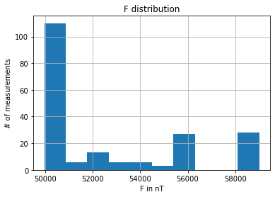
Mapping the GPS Track using the annotated Magnetic Values (optional)
Now we are going to plot the annotated GPS track stored into the MagDataFinal dataframe to see how the different magnetic components in a map to have a better prespective of the impact of the earth magnetic field.
ValidateDF.plot(kind="scatter", x="Latitude", y="Longitude",
    label="Magnetic Intensity in nT",
    c="F", cmap=plt.get_cmap("gist_rainbow"),
    colorbar=True, alpha=0.4, figsize=(10,7),
    sharex=False #This is only needed to get the x-axis label working due to a current bug in pandas plot.
)

plt.ylabel("Longitude", fontsize=12)
plt.xlabel("Latitude", fontsize=10)
plt.legend(fontsize=12)
plt.show()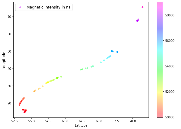
import geopandas
import geoplot
import hvplot.pandas
gdf = geopandas.GeoDataFrame(ValidateDF, geometry=geopandas.points_from_xy(ValidateDF.Longitude, ValidateDF.Latitude))
gdf.head()| Latitude | Longitude | Altitude | TotalPoints | Minimum_Distance | Average_Distance | Kp | N | E | C | N_Obs | E_Obs | C_Obs | H | D | I | F | geometry | |
|---|---|---|---|---|---|---|---|---|---|---|---|---|---|---|---|---|---|---|
| DateTime | ||||||||||||||||||
| 2014-09-08 05:54:00 | 70.854717 | 68.307333 | 0.000 | 46 | 327.950987 | 665.008368 | 1.308696 | 6949.075221 | 3851.112405 | 57703.184834 | 6970.420967 | 3838.494559 | 57689.934814 | 7944.854510 | 28.994810 | 82.160529 | 58247.560062 | POINT (68.30733 70.85472) |
| 2014-09-08 06:10:00 | 70.830300 | 67.975050 | 0.406 | 46 | 340.038476 | 667.146029 | 1.308696 | 6985.622920 | 3866.290909 | 57644.882192 | 7006.455690 | 3854.336448 | 57631.552162 | 7984.180169 | 28.962950 | 82.114343 | 58195.185161 | POINT (67.97505 70.83030) |
| 2014-09-08 06:26:00 | 70.761717 | 67.752417 | 0.498 | 55 | 348.223318 | 678.815409 | 1.190909 | 7035.516299 | 3877.393141 | 57609.773161 | 7053.372261 | 3867.299155 | 57596.673601 | 8033.222713 | 28.859910 | 82.061748 | 58167.161103 | POINT (67.75242 70.76172) |
| 2014-09-08 06:42:00 | 70.686517 | 67.561983 | 0.787 | 55 | 355.472899 | 680.040733 | 1.190909 | 7082.942040 | 3886.893072 | 57574.854667 | 7100.195014 | 3877.501165 | 57561.704322 | 8079.356763 | 28.756578 | 82.011966 | 58138.970542 | POINT (67.56198 70.68652) |
| 2014-09-08 07:14:00 | 70.685450 | 67.548317 | 0.337 | 55 | 355.980432 | 680.062802 | 1.190909 | 7086.053455 | 3888.434162 | 57584.748919 | 7102.154616 | 3880.203863 | 57571.538841 | 8082.825855 | 28.755544 | 82.009936 | 58149.250914 | POINT (67.54832 70.68545) |
gdf.hvplot(title=f'Annotated trajectory using MagGeo - F GeoMag Intensity',
           geo=True,
           c='F',
           tiles='CartoLight',
           frame_width=700,
           frame_height=500)
Unable to display output for mime type(s): gdf.hvplot(title=f'Annotated trajectory using MagGeo - I Inclination',
geo=True,
tiles='CartoLight',
c='I',
cmap='Viridis',
frame_width=700,
frame_height=500)Unable to display output for mime type(s): world = geopandas.read_file(geopandas.datasets.get_path('naturalearth_lowres'))
ax = world.plot(color='white', edgecolor='black', figsize = (12,6))
minx, miny, maxx, maxy = gdf.total_bounds
ax.set_xlim(minx, maxx)
ax.set_ylim(miny, maxy)
# We can now plot our ``GeoDataFrame``.
gdf.plot(ax=ax, column='F', legend=True,
legend_kwds={'label': "Magnetic Intensity in nT",
'orientation': "horizontal"})
plt.ylabel("Longitude", fontsize=9)
plt.xlabel("Latitude", fontsize=9)
plt.show()
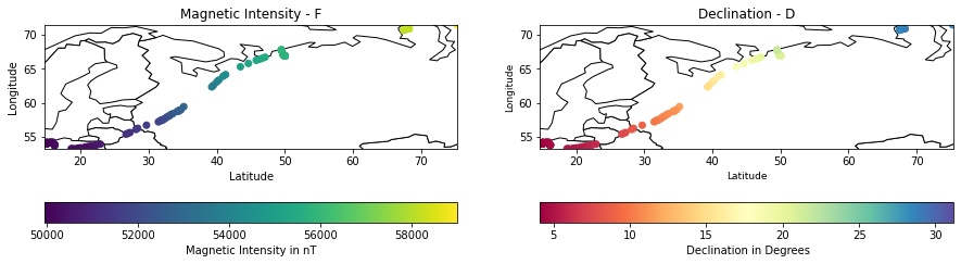
fig, (ax1, ax2) = plt.subplots(ncols=2, figsize = (15,6))

ax1 = world.plot(ax=ax1, color='white', edgecolor='black')
xlim = ([gdf.total_bounds[0],  gdf.total_bounds[2]])
ylim = ([gdf.total_bounds[1],  gdf.total_bounds[3]])
ax1.set_xlim(xlim)
ax1.set_ylim(ylim)


gdf.plot(ax=ax1, column='F', legend=True,
         legend_kwds={'label': "Magnetic Intensity in nT",
                      'orientation': "horizontal"})
plt.ylabel("Longitude", fontsize=9)
plt.xlabel("Latitude", fontsize=9)
ax1.set_title('Magnetic Intensity - F')
ax1.set_xlabel('Latitude')
ax1.set_ylabel('Longitude')


ax2 = world.plot( ax=ax2, color='white', edgecolor='black')
xlim = ([gdf.total_bounds[0],  gdf.total_bounds[2]])
ylim = ([gdf.total_bounds[1],  gdf.total_bounds[3]])
ax2.set_xlim(xlim)
ax2.set_ylim(ylim)


# We can now plot our ``GeoDataFrame``.
gdf.plot(ax=ax2, column='D', legend=True, cmap='Spectral',
         legend_kwds={'label': " Declination in Degrees",
                      'orientation': "horizontal"})
ax2.set_title('Declination - D')
ax2.set_xlabel('Latitude')
ax2.set_ylabel('Longitude')
Text(567.7954545454544, 0.5, 'Longitude')